滤波
滤波操作包括对图像应用具有特定PSF的卷积,以修改图像、增强某些特征或减少某些频率。
在本节中,我们将看到一些滤波器的示例。 首先,我们从常见的滤波器(模糊、边缘检测和锐化)开始,这些滤波器是根据图像域中的分析定义的。 然后,我们继续介绍两个重要的滤波器系列:低通和高通滤波器, 它们是根据傅里叶域中的考虑来定义的。
模糊滤波
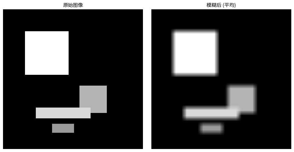
模糊滤波的一个例子在 Figure 1 中给出。 输出图像的每个像素是原始图像中一个窗口内像素强度的平均值。 Figure 1 中的PSF非常简单:
只要PSF定义了一个(可能是加权的)平均值,就可以使用其他尺寸、形状和系数。

Figure 1:模糊滤波。
代码示例设置
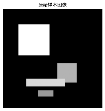
为了演示这些滤波器,我们需要一个样本图像和一些辅助函数。下面的代码块创建了一个带有不同强度矩形的简单合成图像,并提供了一个使用Matplotlib并排显示多个图像的函数。此设置将用于本章中的所有后续示例。
import numpy as np
import matplotlib.pyplot as plt
from scipy.signal import convolve2d
from skimage.draw import rectangle

# 配置中文字体支持
# 按优先级尝试不同的中文字体
plt.rcParams['font.sans-serif'] = ['Noto Sans CJK SC', 'Noto Sans CJK JP', 'SimHei', 'Microsoft YaHei', 'WenQuanYi Micro Hei', 'DejaVu Sans']
plt.rcParams['axes.unicode_minus'] = False  # 解决负号显示问题

# --- 创建一个用于演示的样本图像 ---
sample_image = np.zeros((128, 128), dtype=np.float32)
# 添加一个大方块
start = (20, 20)
extent = (40, 40)
rr, cc = rectangle(start, extent=extent, shape=sample_image.shape)
sample_image[rr, cc] = 1

# 添加一个更小、更暗的方块
start = (70, 70)
extent = (25, 25)
rr, cc = rectangle(start, extent=extent, shape=sample_image.shape)
sample_image[rr, cc] = 0.7

# 添加一些额外的矩形特征
start = (90, 30)
extent = (10, 50)
rr, cc = rectangle(start, extent=extent, shape=sample_image.shape)
sample_image[rr, cc] = 0.85

start = (105, 45)
extent = (8, 20)
rr, cc = rectangle(start, extent=extent, shape=sample_image.shape)
sample_image[rr, cc] = 0.6

# --- 用于绘图的辅助函数 ---
def plot_images(images, titles, figsize=(10, 5)):
    n = len(images)
    fig, axes = plt.subplots(1, n, figsize=figsize)
    if n == 1:
        axes = [axes]
    for ax, img, title in zip(axes, images, titles):
        ax.imshow(img, cmap='gray')
        ax.set_title(title)
        ax.axis('off')
    plt.tight_layout()
    # 在Jupyter Book中,默认情况下会自动显示绘图
    # plt.show()

# 显示原始样本图像
plot_images([sample_image], ["原始样本图像"], figsize=(4, 4))
# 创建一个简单的5x5平均核(方框模糊)
kernel_size = 5
kernel = np.ones((kernel_size, kernel_size)) / (kernel_size**2)

# 应用卷积
blurred_image = convolve2d(sample_image, kernel, mode='same', boundary='symm')

plot_images([sample_image, blurred_image], ["原始图像", "模糊后 (平均)"])
用于边缘检测的导数滤波器
图像中的边缘对应于强度快速变化的区域。在数学上,这些变化可以通过计算图像信号的导数来检测。我们可以使用有限差分来近似这些导数,从而得到用于边缘检测的卷积核。
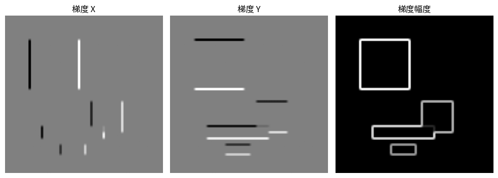
一阶导数(图像梯度)
一阶导数告诉我们变化率。对于二维图像 (g(x,y)),梯度是一个指向最大增长率方向的向量:
我们可以使用卷积核来近似这些偏导数。Sobel算子是一个常见的选择:
用这些核对图像进行卷积,我们得到梯度分量 (g_x) 和 (g_y)。梯度幅度 (||\nabla g|| = \sqrt{g_x^2 + g_y^2}) 给出了边缘强度。
# 用于近似导数的Sobel核
sobel_x = np.array([[-1, 0, 1], [-2, 0, 2], [-1, 0, 1]])
sobel_y = np.array([[-1, -2, -1], [0, 0, 0], [1, 2, 1]])

# 计算梯度分量
grad_x = convolve2d(sample_image, sobel_x, mode='same', boundary='symm')
grad_y = convolve2d(sample_image, sobel_y, mode='same', boundary='symm')

# 计算梯度幅度
grad_magnitude = np.sqrt(grad_x**2 + grad_y**2)

plot_images([grad_x, grad_y, grad_magnitude], ["梯度 X", "梯度 Y", "梯度幅度"])
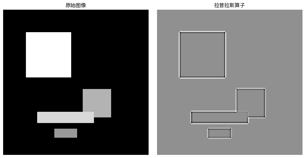
二阶导数(拉普拉斯算子)
二阶导数测量信号的曲率。在图像中,拉普拉斯算子可以通过寻找零交叉点(信号曲率从凹变为凸或反之的地方)来找到边缘,这通常发生在边缘处。拉普拉斯算子定义为:
一个常用于近似拉普拉斯算子的核是:
# 拉普拉斯核
laplacian_kernel = np.array([[0, 1, 0], [1, -4, 1], [0, 1, 0]])

# 应用拉普拉斯算子
laplacian_image = convolve2d(sample_image, laplacian_kernel, mode='same', boundary='symm')

plot_images([sample_image, laplacian_image], ["原始图像", "拉普拉斯算子"])
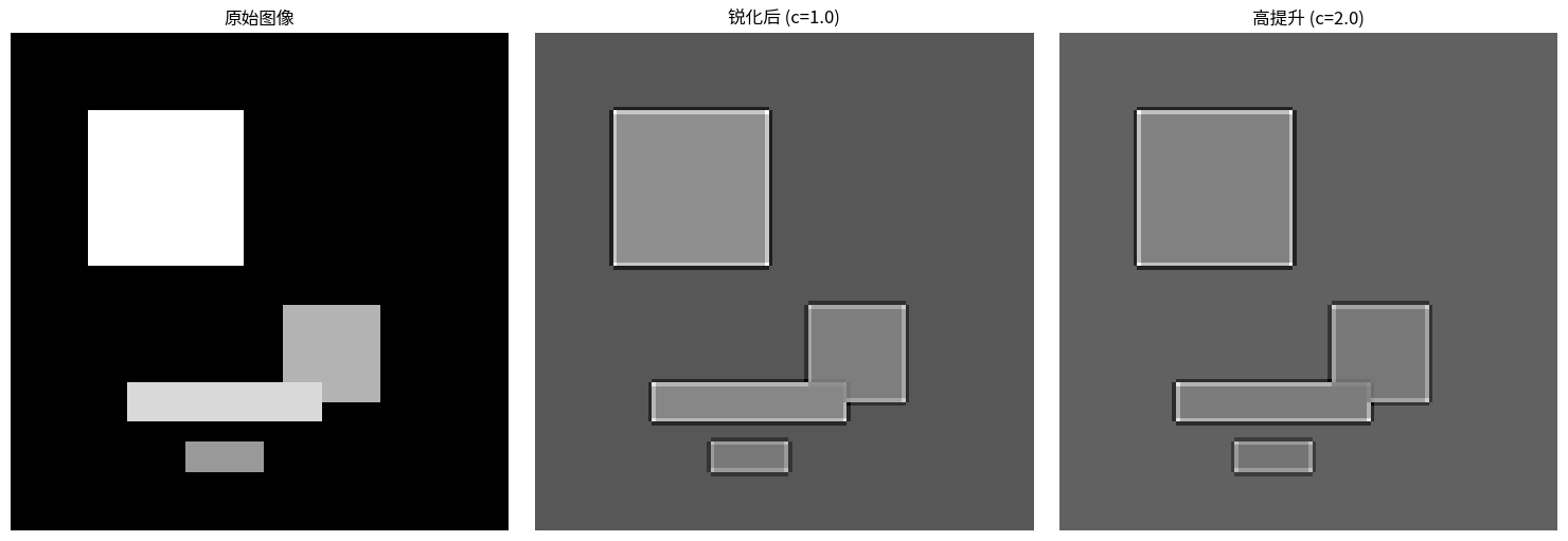
锐化滤波
锐化滤波增强了图像中的边界。 它可以通过从原始图像中减去拉普拉斯算子来计算。这样做的效果是将拉普拉斯算子捕捉到的高频细节添加回图像中。
这个操作的核就是单位矩阵减去拉普拉斯核:

Figure 2:锐化滤波。
# 锐化核是通过将负的拉普拉斯算子添加到单位核上来创建的。
sharpen_kernel = np.array([[0, -1, 0], [-1, 5, -1], [0, -1, 0]])

# 应用锐化核
sharpened_image = convolve2d(sample_image, sharpen_kernel, mode='same', boundary='symm')

plot_images([sample_image, sharpened_image], ["原始图像", "锐化后"])
低通滤波
因为滤波是图像与特定PSF的卷积, 所以它也可以通过将图像的DFT与PSF的DFT相乘来实现。 这样就可以在傅里叶域而不是空间域中定义滤波器。
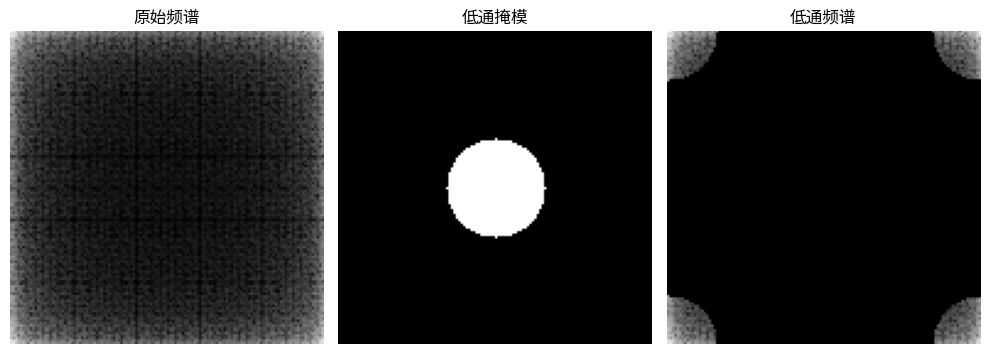
Figure 3 显示了一个低通滤波的例子。 第一行显示了空间域中的滤波(卷积), 第二行显示了傅里叶域中的相同信息, 其中滤波后图像的DFT是原始图像的DFT与PSF的DFT的(逐点)乘积。
低通滤波只保留低频,从而产生模糊的图像。

Figure 3:低通滤波示例:只保留低频。 顶行:空间域,底行:DFT的幅度 (为简洁起见,未显示相位)。
类似地,上面定义的模糊滤波器也是一个低通滤波器。
高通滤波
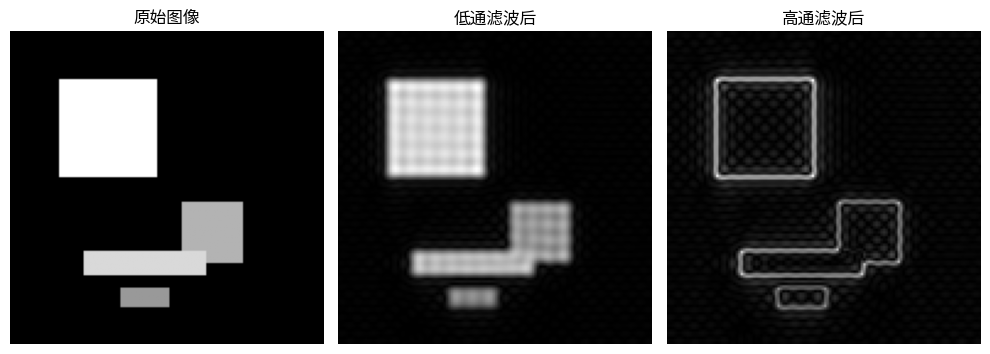
与低通滤波相反,高通滤波只保留高频, 即强度的突然变化(Figure 4)。

Figure 4:高通滤波示例:只保留高频。 顶行:空间域,底行:DFT的幅度 (为简洁起见,未显示相位)。
类似地,上面定义的导数滤波器也是高通滤波器。
# --- 频域滤波 ---
from numpy.fft import fft2, ifft2, fftshift, ifftshift

# 计算图像的二维FFT
fft_image = fftshift(fft2(sample_image))

# 创建一个低通滤波器(一个圆形掩模)
rows, cols = sample_image.shape
crow, ccol = rows // 2 , cols // 2
radius = 20
mask = np.zeros((rows, cols), np.uint8)
center = (crow, ccol)
r, c = np.ogrid[:rows, :cols]
mask_area = (r - center[0])**2 + (c - center[1])**2 <= radius*radius
mask[mask_area] = 1

# 应用掩模进行低通滤波
fft_low_pass = fft_image * mask
low_pass_image = np.abs(ifft2(ifftshift(fft_low_pass)))

# 应用掩模进行高通滤波(掩模的反转)
fft_high_pass = fft_image * (1 - mask)
high_pass_image = np.abs(ifft2(ifftshift(fft_high_pass)))

# 显示结果
plot_images(
    [fftshift(np.log(1+np.abs(fft_image))), mask, fftshift(np.log(1+np.abs(fft_low_pass)))],
    ["原始频谱", "低通掩模", "低通频谱"]
)
plot_images(
    [sample_image, low_pass_image, high_pass_image],
    ["原始图像", "低通滤波后", "高通滤波后"]
)